Actuarial GLM Pricing using Metropolis MCMC
This week I will present some material on using the Metropolis-Hastings algorithm to carry out GLM-like actuarial pricing in R. We use the motorins data set from
the faraway package and compare the output with using a standard glm() function in R.
Monte Carlo methods are pretty popular nowadays particularly for analytically intractable problems however we will present a simple model. The paper by Chib and
Greenberg outlines the Metropolis-Hastings method. In this as assume a poisson likelihood and a normal prior for the beta coefficients N(0, 10), we use a multivariate
normal distribution as our proposal distribution and we sample from this using the mvrnorm() function from the
MASS package.
An initial variance for the proposal distribution is given by:
mPopVariance <- as.numeric(var(log(dObs/dExposure + .5)))*solve(t(dDesign) %*% dDesign)
There are a few things to note here. Firstly, we have to adjust the observed counts dObs with the exposure dExposure, and the design matrix is dDesign. Note the design
matrix can be obtained using the model.matrix() function. This is appropriate as a “first pass” but as we will later see, variance adaptation methods are required to properly explore the posterior distributions.
Note also that when calculating the density for the poisson distribution, you need to adjust for the exposure:
dpois(dObs, dExposure*exp(dDesign %*% betaProposal))
I will be running the equivalent of this model:
glm(Claims ~ Kilometres + Zone + Bonus + Make, data = motorins, family = poisson(link = "log"), offset = log(motorins$Insured))
The Bonus variable needs to be converted to a factor before the analysis is carried out.
Outputs
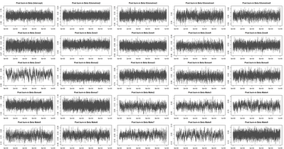
In this analysis we allow for 4000 iterations for burn-in and collect a further 10,000 iterations. The raw outputs show that the burn-in used is appropriate.
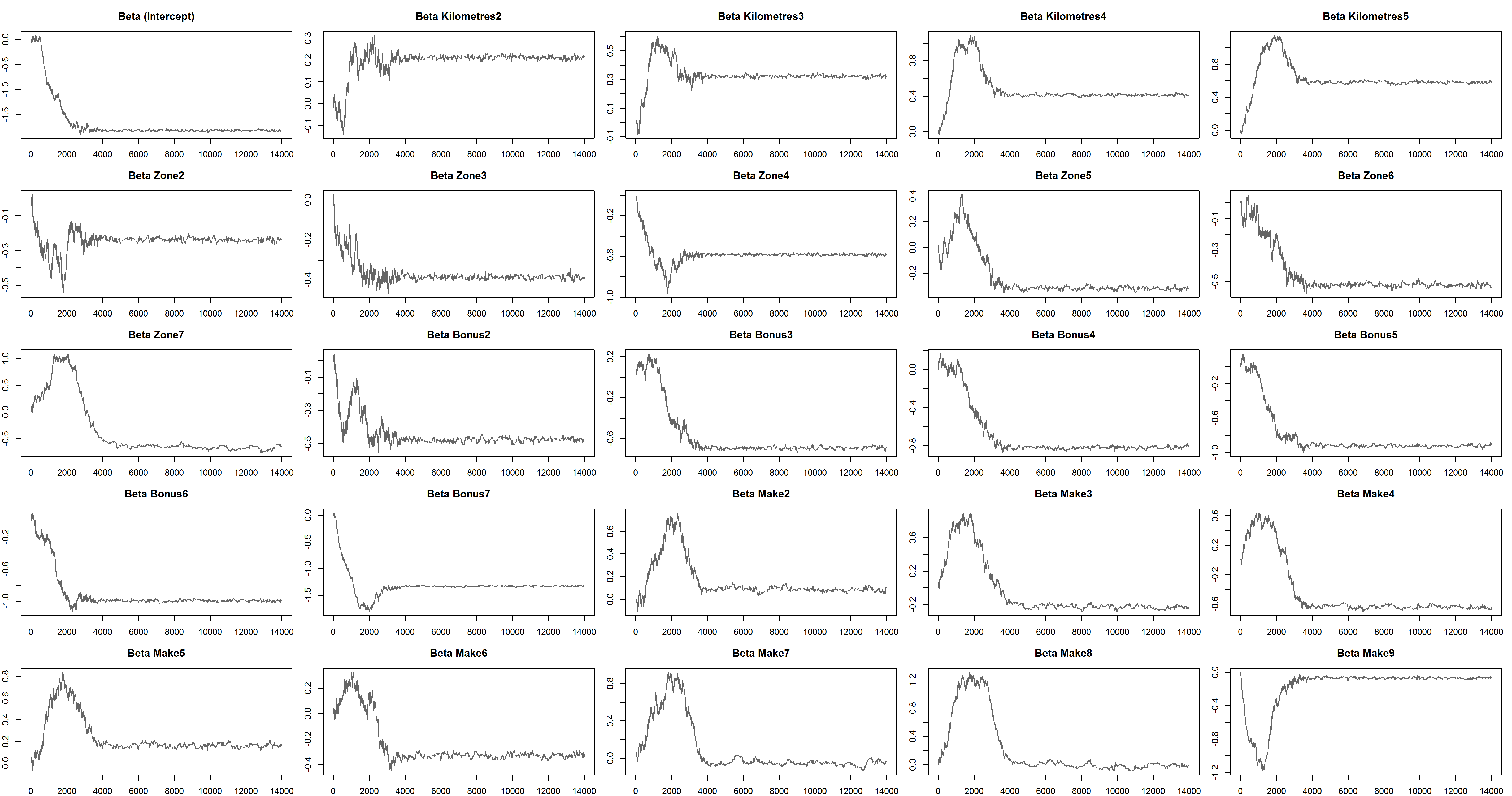
A closer look at the chain output shows that the posterior distribution is not being properly explored. At this point our post-burning acceptance probability is 0.055, much lower than the rule of thumb for multivariate distributions 0.234 {Roberts et al}.
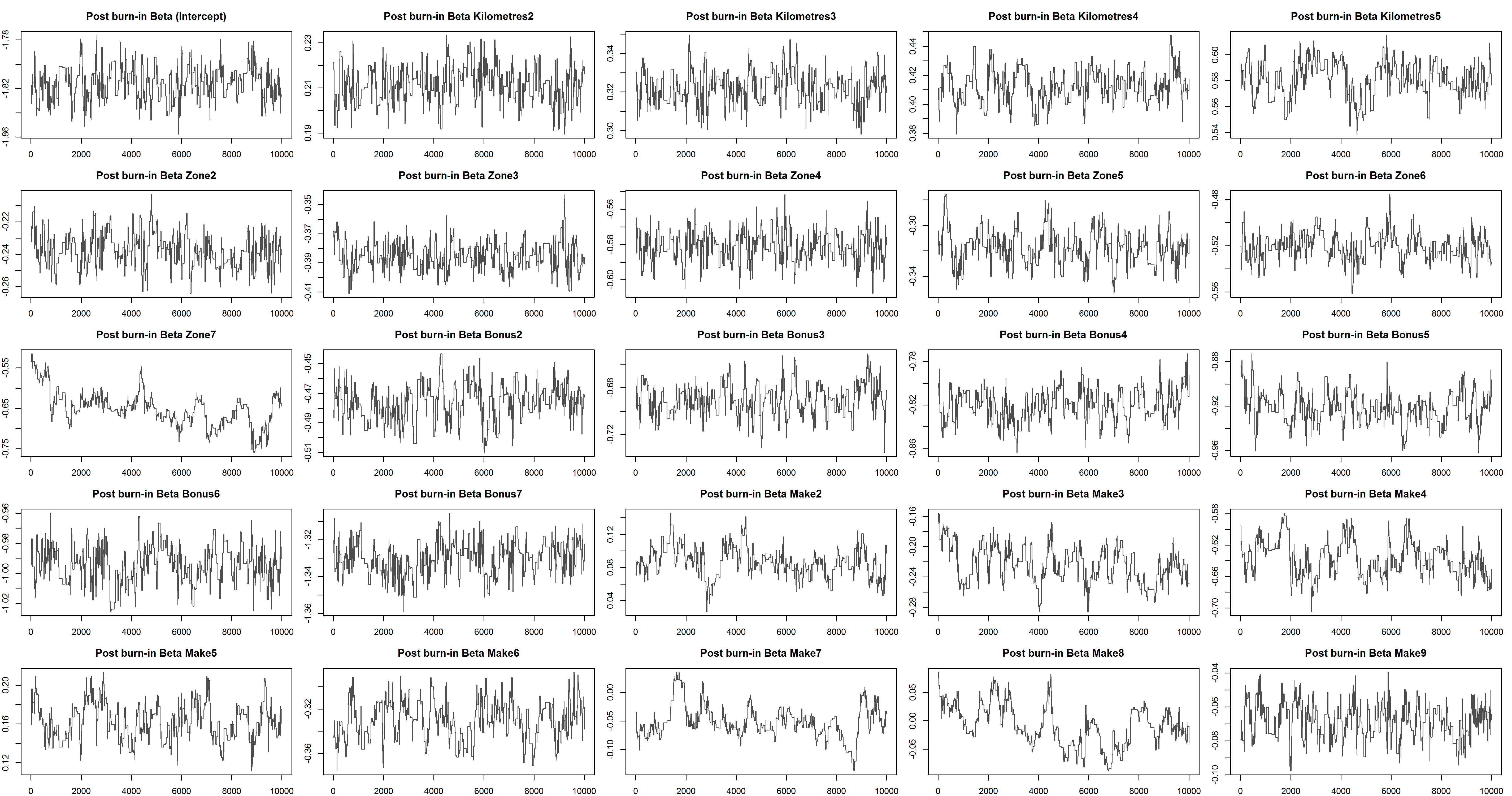
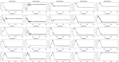
We can easily create an adaptive scheme for the sampling variance that keeps the acceptance probability hovering around where it should be. Doing this gives the full burn-in chart below:
And the post burn in chart below.
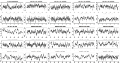
Now we bump the number of simulations to 100,000. The full and post burn in charts are given below. The acceptance probability was 0.257 after setting a target of 0.25 on the variance adapting algorithm.

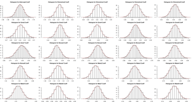
Below we show the histogram and density line (grey) for the post burn-in chain and compare this with the output from the glm() function summary for the coefficient distribution (red).
Conclusion
MCMC methods applied to generalized regression model schemes give us the opportunity to analyse analytically intractable problems, the simple one tackled here shows that there can be many challenges while using this technique. The proposal variance algorithm was applied post burn-in. It is possible to obtain faster convergence by investigating different burn-in variance modification schemes. If we are interested in reducing the dependence withing samples it may be useful to considering “thinning” obtained sample and use the acf() function as a guide. The great disadvantage here of course is that > 70% of the proposed samples are thrown away post burn-in, which seems wasteful from a resource point of view. Properly formulated Gibbs sampling schemes can over come this. I hope that this has been useful.
References
- S. Chib and E. Greenberg, Understanding the Metropolis-Hastings Algorithm, The American Statistician, 1995, Vol. 49, No. 4, p 327-335
- G. O. Roberts, A. Gelman, W. R. Gilks, Weak Convergence and Optimal Scaling of Random Walk Metropolis Algorithms, The Annals of Applied Probability, Vol. 7, No. 1 (Feb., 1997), pp. 110-120.