Claims reserving using nonlinear regression and state space models
The ChainLadder R package provides traditional tools for projecting the ultimate loss of a book of business. Here we outline outputs from a nonlinear regression model and a state space model. The data used in this presentation was obtained from the auto claims in the ChainLadder package. In addition Markus Gesmann’s blog also details GLM methods in Reserving, the first of a three part blog entry is located here. For those interested in Hierarchical growth models for loss reserving, a very good paper by James Guszcza is given here.
This research will be discussed in detail in my presentation at the R In Insurance conference 2013.
Fitting cumulative losses using nonlinear regression in R
Many curves can be used to fit cumulative losses, here we outline the fit for the Gompertz curve. The equation for the Gompertz curve is given by:
\( P_t = \alpha e^{-\beta e{-\gamma t}} \qquad \ldots (1) \)
Nonlinear least squares can be used to fit the parameters of the curve to cumulative losses. To do this we need good starting parameters for the least squares algorithm. These can be obtained from approximates given by Franses. We take the logarithm of equation (1), giving:
\( X_t = \log(\alpha) -\beta e^{-\gamma t} \)
\( Z_t = X_t - X_{t-1} \)
\( Z_t = e^{-\gamma t}(e{-\gamma} - 1)\beta \)
then \(\gamma\) can be obtained using linear regression with
\( \log(Z_t) = -\gamma t + \log(A) \)
We can then estimate \(\gamma\) using equation (1) and \(\beta\) using
\(\beta = \frac{A}{e^{\gamma} - 1}\) and obtain \(\alpha\) using
\(\alpha = \log(P_t) + \beta e^{-\gamma t}\)
Next we can fit the curves using nonlinear regression to obtain parameters. The plot of the cumulative claims and the fitted curve is shown below.
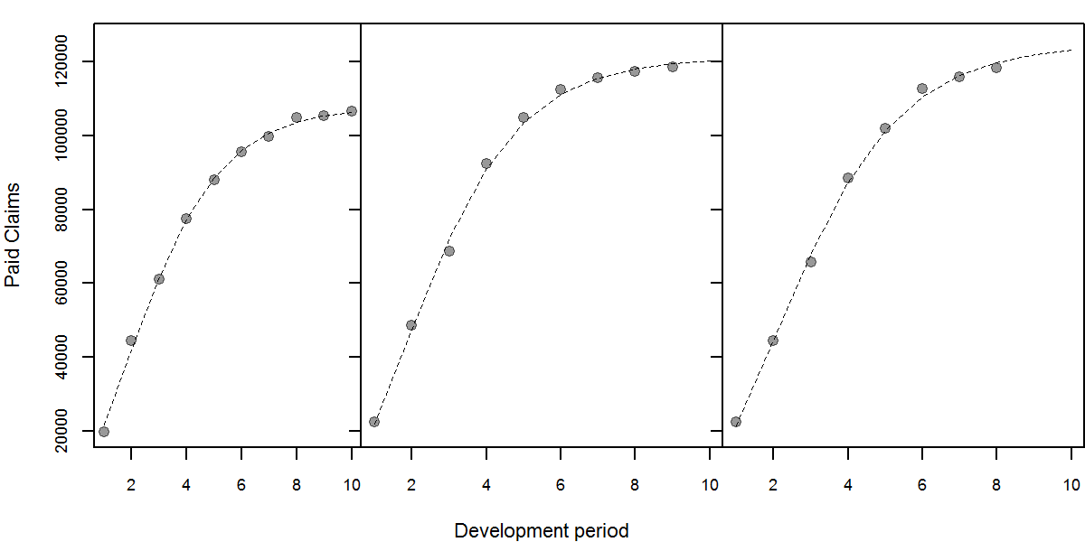
Figure showing the cumulative claims and the fitted curves. Curves are projected to the 10th development period.
We can overlay the confidence interval band of the fit using:
\(f(x_0, \hat{\theta}) \pm s | v^{T}0 R^{-1}{1} | t(N - P, \frac{\alpha}{2}) \)
\(R\) is obtained from the \(QR\) decomposition of \(X = QR\)
\(v_0\) is the gradient
\(s\) is the standard deviation of the random error
\(t(N-P, \frac{\alpha}{2})\) is the quantile obtained from the t-distribution and \( (N - P)\) degrees of freedom at probability of freedom at \(\alpha\) significant level. [Bates & Watts]
The plot of the cumulative claims, the fitted curves and the confidence intervals are shown below.
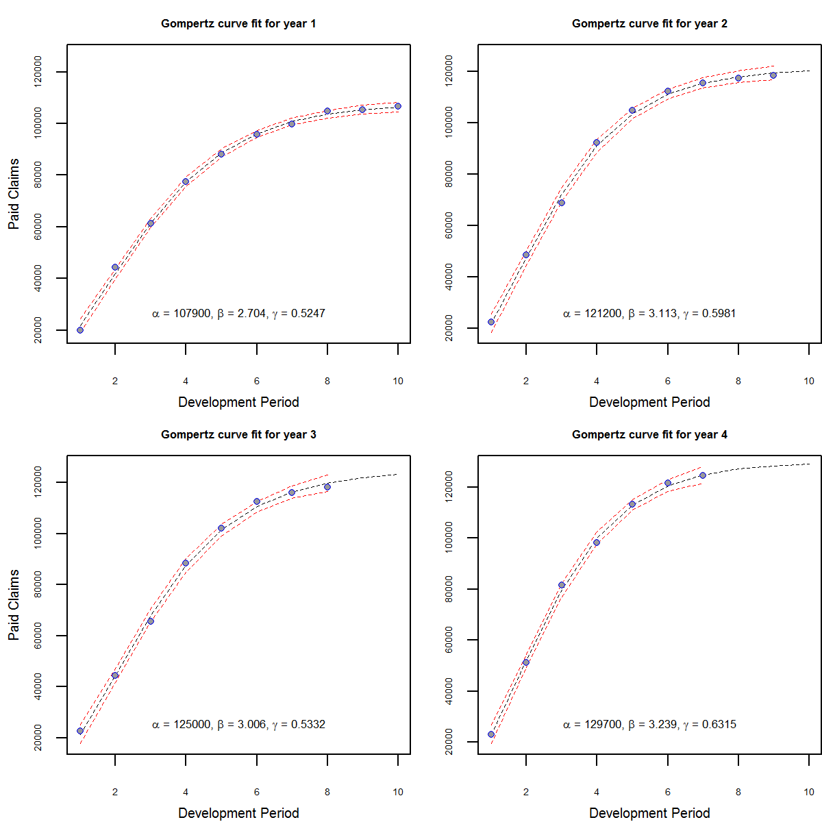
Figure showing cumulative claims with nonlinear regression fit and 95% confidence interval for the fitted points. The fitted model is used to project the subsequent years to the 10th development period.
Filtered cumulative claims using state space models
The confidence interval above indicate error of the model fit and not the uncertainty associated with the claims development process. State space models give us a formal frame work that allows us to calculate the predictive distribution of the claims development given certain assumptions on the dynamic process of claims development.
Dynamic linear models are charaterized by the set \({F_t, G_t, V_t, W_t}\), these relate observations \(Y_t\) to the state vector \(\theta_t\) through time. The dlm R package can be used to carry out the calculation. The observations and states are conditionally independent:
$$ (Y_t | \theta_t) \sim N(F^{\prime}_t \theta_t, V_t) $$
$$ (\theta_t | \theta_{t-1}) \sim N(G_t \theta_{t-1}, W_t) $$
These can be written as observation and state or system equations:
observation equations: \( \quad Y_t = F^{\prime}_t \theta_t + v_t, \qquad v_t \sim N(0, V_t) \)
system equations: \(\quad \theta_t = G_t \theta_{t-1} + w_t, \qquad w_t \sim N(0, W_t)\)
prior distribution: \(\quad (\theta_0 | D_0) \sim N(m_0, C_0)\)
We can compute the distribution of the state
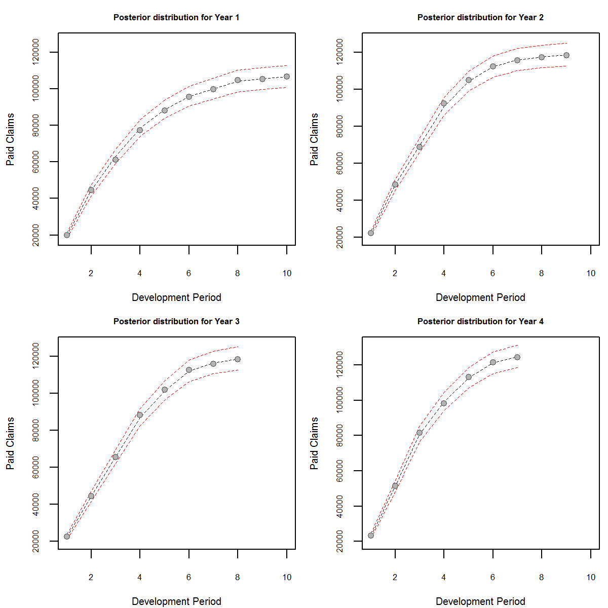
Figure Showing the filtered distribution with 95% confidence interval
The advantage of the method is that we have computed the posterior claims distribution of the states from which inference can be done. We can also calculate the forecast claims distributions:
\( f_t(k) = F_{t + k}^{\prime} G^{k}m_{t} \)
\( Q_t(k) = F_{t + k}^{\prime} R_t F_{t + k} + V_{t + k} \)
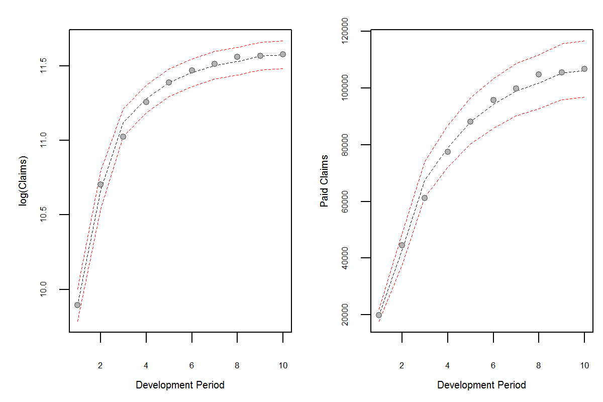
Figure showing the step ahead claims forecast distribution with 95% confidence interval.
Conclusion
State space models can provide ready parametric outputs to claims distributions, they give modelers the opportunity to qualify evolution error in the process as well as observational error. The evolution error can be used to model increased uncertainty of claims and allow our forecasts to become more adaptive. They also provide a formal structure to intervene when we have new information that could be useful in preempting future observations. The method used here is based on parameters from nonlinear regression but other authors have tackled this subject previously [De Jong, Verrall].
References
- Gesmann M., Daniel M. and Zhang W. ChainLadder R package.
- Franses, P. H., Fitting a Gompertz Curve, The Journal of the Operational Research Society, Vol 45, No. 1 p109-113.
- Bates, D. M. and Watts D. G., Nonlinear regression analysis and its applications.
- West M., Harrison J., Bayesian Forecasting and Dynamic Models, Springer Series in Statistics.
- Petris G. the dlm R package.
- De Jong P. and Zehnwirth B., Claims reserving, state space models and the kalman filter, Journal of the Institute of Actuaries, Vol. 110, 1983, p157-181.
- Verrall R. J., A state space representation of the chain ladder linear model, Journal of the Institute of Actuaries, Vol. 110, 1989, p589-609.